
Next step to apply abstraction and functional approach to drawing lines with special properties.
Characteristics of line: start, end points and path between. Anything can happen along line as random or other factors are applied to it.
Underlying path across a grid of pixels and problems drawing it: Bresenham's algorithm.
Abstracting error-value checking to a closure - simple implementation, optimization.
Writing a function to draw a line between any two points, any width with a colour gradient along its length: needs end points of lines normal to conceptual underlying line.
Writing another closure to return maximum-width end-points of lines at points along underlying length. Problem: filling in missing pixels between adjacent lines due to jagged profile when they offset along underlying line.
Program draws colour gradient lines.
Applying similar closure approach to diverse grids: circular and random spaced grid using array.
PROGRAM 3D grid and thistle-down blob drawn with colour grad lines, moves along its length.
Mostly code: say 48 hours work, 2 weeks max. Time to post code on blogger????
Tuesday, 28 April 2009
Thursday, 9 April 2009
In Search of Processings Lost
As you may have noticed, Processing programs that use random() and/or noise() and do not set the seed for these functions before they are called, create a different output for each run. The run that gets the superb effect is lost forever but setting seeds always gets the same old effect as the last time. To retain random creation and the capability of recreating a successful run it would nice if the value of seeds could be read at the beginning of a run and stored for future reference. Unfortunately this is not possible - the underlying Java Random class sets seed randomly from its () constructor and does not include a method for retrieving a value that can be used with setSeed().
A workaround is to generate a value for seed using a similar procedure to Random's, record it, and then pass it to a seed setter:
If this run turns out to be the great one change setup() to
identical graphic output is recreated. Otherwise, just continue with the original setup() version and hope for the best. The same seed generation method is appropriate for noiseSeed(). The seed calculation shown will avoid holes in the total sequence of values returned by nextLong() - if such exist and affect the 48 bit seed used by Random that is.
A workaround is to generate a value for seed using a similar procedure to Random's, record it, and then pass it to a seed setter:
void setup() {
   size(WIDTH, HEIGHT);
   long seed = 8682522807148013L + System.nanoTime();
   System.out.println(seed);
   randomSeed(seed);
   doDrawing();
}

output: 8702777365341749
If this run turns out to be the great one change setup() to
void setup() {
   size(WIDTH, HEIGHT);
//      long seed = 8682522807148013L + System.nanoTime();
//      System.out.println(seed);
   randomSeed(8702777365341749L);
   doDrawing();
}
identical graphic output is recreated. Otherwise, just continue with the original setup() version and hope for the best. The same seed generation method is appropriate for noiseSeed(). The seed calculation shown will avoid holes in the total sequence of values returned by nextLong() - if such exist and affect the 48 bit seed used by Random that is.
Thursday, 26 March 2009
Drawing with Lines
This Chapter examines the nature of lines and how they can be used to create art using the line drawing facilities provided by Processing. Initially we look at the broadest possible description of a line and then get down to the nitty-gritty of making a program produce a required result by drawing lines.
Not all lines are straight. A geodesic, the shortest distance between two points on the surface of the Earth, is a curve. Add random noise to a line and it can take on an aspect of a lightning strike, flickering flames, a rough sea, rain falling on a lake and other representations of chaotic behaviour or liquid flow according to the frequencies present in the noise. Any kind of line, straight, curved or distorted, can suggest an edge, a boundary or a link between two locations.
Alternatively we may want a simplified view where the purity of straight lines or the intersections of many lines are used to represent underlying curvature or some more complex shape. A grid of lines can define a two or three dimensional space where equal spacing represents the world as we see it but other spacings can give the effect of non-linearity. We can show distances and dimensions that would otherwise be too small or too large to see. We can also employ the additional dimensions of light, colour, hardness, discontinuity (dots and dashes) and blur to achieve the effect we want.
There are few straight lines in nature and even fewer orthogonal straight lines. A straight line has its own special significance when used representationally. An icon of human-kind one might say.
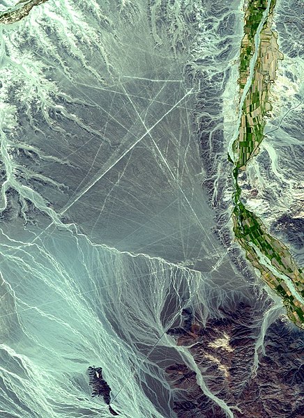
Satelight image of the nazca lines
from Wikimedia Commons NASA/GSFC/MITI/ERSDAC/JAROS, and U.S./Japan ASTER Science Team
Not all lines are straight. A geodesic, the shortest distance between two points on the surface of the Earth, is a curve. Add random noise to a line and it can take on an aspect of a lightning strike, flickering flames, a rough sea, rain falling on a lake and other representations of chaotic behaviour or liquid flow according to the frequencies present in the noise. Any kind of line, straight, curved or distorted, can suggest an edge, a boundary or a link between two locations.
Alternatively we may want a simplified view where the purity of straight lines or the intersections of many lines are used to represent underlying curvature or some more complex shape. A grid of lines can define a two or three dimensional space where equal spacing represents the world as we see it but other spacings can give the effect of non-linearity. We can show distances and dimensions that would otherwise be too small or too large to see. We can also employ the additional dimensions of light, colour, hardness, discontinuity (dots and dashes) and blur to achieve the effect we want.
There are few straight lines in nature and even fewer orthogonal straight lines. A straight line has its own special significance when used representationally. An icon of human-kind one might say.
Satelight image of the nazca lines
from Wikimedia Commons NASA/GSFC/MITI/ERSDAC/JAROS, and U.S./Japan ASTER Science Team
The Line Drawing Functions
Having got to grips with coordinates, setting colours and suchlike you will probably find line drawing relatively simple. Unlike some less enlightened environments Processing has only a single line drawing function and three line attribute setters.
The line() function
Line(), is overloaded for drawing in 2D and in 3D. A line function with four arguments draws a line on the picture plane, the screen for current purposes.
draws a line from the point (x1, y1) to (x2, y2).
To draw in 3D we must first setup a 3D drawing environment. Two 3D environments are available and as detailed in XXXX they are invoked by passing an extra argument to the function that sets the window size at the start of the program. You can use either
With a 3D environment in place use:
The line() functions accept floating point values and can be called with floating point or integer coordinates. Fractional values are rounded to the nearest pixel but casting arguments to integer can be sometimes be useful to smooth jagged parallel line endings e.g:
Line attribute setters
Three functions set the 'style' of the line that will be drawn by the next and subsequent calls to line(). The effect of calling any one of these functions remains in place until the same function is called again. To be able to revert to a previous value we need to make sure the old values are stored. Line style setters and many other functions that modify the drawing environment have a corresponding variable in the current instance of the Processing application interface, called 'g'. To store the current line colour, for example, we can write
The stroke() line colour setter accepts the same colour and alpha opacity values as the other Processing colour setters detailed earlier in XXXXX. Two other setters affect line drawing: strokeWeight() sets line thickness, strokeCap() the shape or relative location of the end of a line. The program in Listing CC.1 demonstrates the effect of the line style setters.
Listing CC.1
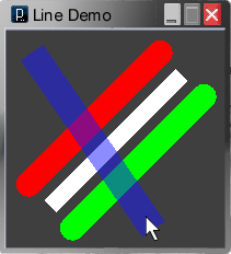
Figure CC.2 Listing CC.1 running.
Running the program note the effect of the attribute setter functions strokeWeight() and strokeCap() for changing line thickness and the shape or relative location of the end of a line as shown in Figure CC.1. Use the mouse to move the blue line over the other lines and note alpha transparency generally and where the lines intersect. Graphics behind an area of transparent colour may appear lighter or darker according to relative brightness values. Try changing the blue line to white, stroke(255, 255, 255, 255 / 2); colours behind are now lightened.
The line() function
Line(), is overloaded for drawing in 2D and in 3D. A line function with four arguments draws a line on the picture plane, the screen for current purposes.
line(x1, y1, x2, y2)
draws a line from the point (x1, y1) to (x2, y2).
To draw in 3D we must first setup a 3D drawing environment. Two 3D environments are available and as detailed in XXXX they are invoked by passing an extra argument to the function that sets the window size at the start of the program. You can use either
size(x, y, P3D); or size(x, y, OPENGL);size() can also be called with a P2D argument to get faster 2D drawing than the default JAVA2D environment provides: size(x, y, P2D). At the time of writing P2D did not support all the facilities of the default mode for line drawing. Try its effect using the simple line drawing program we come to in a moment and check the line drawing and attribute setter functions on the Processing website for current details.
With a 3D environment in place use:
line(x1, y1, z1, x2, y2, z2);to draw a line between points (1) and (2) in three dimensional space. The extra coordinates z1 and z2 are the distances of points behind the picture plane. Their depth back from the front face of the screen is another way of thinking about it. If a line is located behind the picture plane and/or tilted in the depth dimension, it will be shown shorter than its length drawn flat on the screen.
The line() functions accept floating point values and can be called with floating point or integer coordinates. Fractional values are rounded to the nearest pixel but casting arguments to integer can be sometimes be useful to smooth jagged parallel line endings e.g:
line(floatX1, floatY1, (int)floatX2, (int)floatY2); // smooth endings at X2, Y2
Line attribute setters
Three functions set the 'style' of the line that will be drawn by the next and subsequent calls to line(). The effect of calling any one of these functions remains in place until the same function is called again. To be able to revert to a previous value we need to make sure the old values are stored. Line style setters and many other functions that modify the drawing environment have a corresponding variable in the current instance of the Processing application interface, called 'g'. To store the current line colour, for example, we can write
int oldColour = g.strokeColor.Accessing variables using 'dot' notation is discussed later, particularly in Chapter ZZ: Object Oriented Programming. To revert to the old colour write
stroke(oldColour);The facility to store and to revert to old settings allows a section of code or a function to draw using settings applicable to the task in hand and restore old settings afterwards - an aid to abstraction discussed later in this Chapter in connection with parametric graphics.
The stroke() line colour setter accepts the same colour and alpha opacity values as the other Processing colour setters detailed earlier in XXXXX. Two other setters affect line drawing: strokeWeight() sets line thickness, strokeCap() the shape or relative location of the end of a line. The program in Listing CC.1 demonstrates the effect of the line style setters.
      /* set window size and drawing environment */

   // declaring constants static final makes sure they
   // cannot be altered by mistake later in the program
   static final int WIDTH = 200;
   static final int HEIGHT = 200;
   static final int OS = 20; // lines offset from edges

   void setup() {
      // size(WIDTH, HEIGHT, P2D);
      // PD2 mode not fully functional in Processing 1.0.2
      // so use:
      size(WIDTH, HEIGHT);
   }

   /* draw in continuous mode */
   void draw() {
      // fill the window with charcoal grey
      background(0.25 * 255);

      /* draw a 45 deg line top-right to bottom-left */
      // set line colour to greyscale white
      stroke(255);
      // set line width to 12 pixels
      strokeWeight(15);
      // make the ends of the line squared off
      strokeCap(SQUARE);
      // draw the line
      line(WIDTH - 2*OS, 2*OS, 2*OS, HEIGHT - 2*OS);

      /* draw two lines same length, parallel to it */
      // rounded ends
      strokeCap(ROUND);

      /* draw a red line 20 pixels wide above */
      strokeWeight(23);
      stroke(255, 0, 0);  // colour red
      line(WIDTH - 3*OS, OS, OS, HEIGHT - 3*OS);

      /* draw a green line 20 pixels wide below */
      stroke(0, 255, 0);  // colour green
      line(WIDTH - OS, 3*OS, 3*OS, HEIGHT - OS);

      /* draw a blue line 50% opaque, width 20,
         top-left to the mouse cursor */
      stroke(25, 25, 255, 255 / 2);
      strokeWeight(25);
      // extend line past cursor point
      strokeCap(PROJECT);
      line(30, 30, mouseX, mouseY);
   }
Listing CC.1

Figure CC.2 Listing CC.1 running.
Running the program note the effect of the attribute setter functions strokeWeight() and strokeCap() for changing line thickness and the shape or relative location of the end of a line as shown in Figure CC.1. Use the mouse to move the blue line over the other lines and note alpha transparency generally and where the lines intersect. Graphics behind an area of transparent colour may appear lighter or darker according to relative brightness values. Try changing the blue line to white, stroke(255, 255, 255, 255 / 2); colours behind are now lightened.
Parametric Grids
The effect of drawing a single line tends to be minimal and it is more likely that many lines will be needed to produce a required effect. In this section we look at a strategy for doing this that extends the repetition facility provided by loops.
Another name for arguments is parameters and parametric graphics is a common feature of vector graphics applications. Using this approach a drawing task is abstracted (taken out) from the main part of the program and done by passing arguments to a function that draws the graphic. Many similar objects can be drawn with different sizes, locations, colours, and other properties determined by values passed to arguments.
Initially we experiment with parametric grids and to do this with a minimum of work the initial step is to set up a basic grid drawing program for testing them out. Optionally the basic structure can be extended to produce actual drawings that include grids. Listing CC.2 shows the outline:
  /* set window size and drawing environment */

  static final int WIDTH = 900;
  static final int HEIGHT = 600;

  void setup() {
     size(WIDTH, HEIGHT); // default environment
     doDrawing();
  }

  /* draw the drawing */

  void doDrawing() {
     // charcole grey background, again!
     background(0.25 * 255);
     // white grid lines
     stroke(255);
     // one pixel wide
     strokeWeight(1);

     // draw a grid with number of cells xCells * yCells
     int xCells = 13;
     int yCells = 19;
     drawGrid(0, 0, WIDTH, HEIGHT, xCells, yCells, true);

  }

  void drawGrid(int left, int top, int width, int height, int  xCells,
        int yCells, boolean drawOutline){

  }
Listing CC.2
As it stands the outline will compile and run but does nothing except opening a window with a grey background. Sections of functionality will be factored off using calls to drawGrid()to draw as many different grids as we require. Such power should be used carefully so the first thing is to decide exactly what we want a drawGrid() function to do and make sure all drawGrids variations we write do just that.
Arguments left and top are where the top-left corner of the grid will be positioned. Width and height specify the size of the grid in pixels, xCells and yCells the number of areas the grid is divided into in the horizontal and vertical directions respectively. Cells are to be made to fit the grid exactly by distributing any odd pixels evenly across cell widths and heights. If draw outline is passed true a one pixel wide line is to be drawn around the grid within the size given. All this sounds complicated but is actually very easy when we divide up the work using functions.
Drawing grids in 2D
The code for a 2D drawGrid() can be something like this:
Listing CC.3
void drawGrid(int left, int top, int width, int height, int  xCells,
              int yCells, boolean drawOutline){

   // precondition for drawing the grid
   if (width <= 0 || height <= 0) return;

   // compute the coordinates of the rightmost an bottom pixels
   int right = left + width - 1;
   int bottom = top + height - 1;

   // draw the grid
   drawVertGrid(left, top, right, bottom, width, xCells);
   drawHorzGrid(left, top, right, bottom, height, yCells);

   if (drawOutline){
      // save current line width
      float curWeight = g.strokeWeight;
      // draw outline with a line 1 pixel wide
      strokeWeight(1);
      line(left, top, right, top);
      line(right, top, right, bottom);
      line(right, bottom, left, bottom);
      line(left, bottom, left, top);
      // restore line width
      strokeWeight(curWeight);
   }
}
Preconditions for execution
Writing functions it is wise to check that all possible values passed as arguments can be dealt with by the code in the function body. What happens, for example, if drawGrid() is called with zero or negative dimensions passed to width and/or height?
If we see there is a problem a number of options are available. In this case a fully justifiable option is to simply ignore it. We are not trying to create a flawless machine and an emergent property of a program may turn out to be a spectacular work of art. On the other hand, if the code simply does not work a lot of time can be wasted trying to track down the bug.
Another option is to pass the problem on to other functions. Perhaps the grid will be drawn with all or part of it off the screen. This eventuality can be passed on for line() to deal with.
The third option is to write code at the start of the function that checks input is within range. These checks are known as preconditions: execution of other code in the function body is conditional on the checks being passed. There are three ways of dealing with a failed precondition: the function can return immediately to the caller; likewise but it returns a Boolean or some other value indicating success or failure; alternatively an error condition can be created. Java error conditions are dealt with by throwing and catching exception objects, certainly beyond the scope of this Chapter. For drawing grids a simple conditional return statement is appropriate:
if (width <= 0 || height <= 0) return;
Note that other problems such as zero or negative numbers of cells are passed on to the grid-line drawing functions.
Minimizing coding
Another useful strategy is to avoid writing code that does the same thing more than once. This makes the code run faster but more importantly can make it shorter and easier to read. We are going to draw numerous lines from the left to the right of the grid and from its top to the bottom so compute right and bottom before doing anything else:
      int right = left + width - 1;
      int bottom = top + height - 1;
The next task is to draw the gridlines, done by two functions:
drawVertGrid(left, top, width, bottom, xCells, constrain);Finally a one pixel wide outline is drawn around the grid if this option is set having first saved the current line thickness, as shown in Listing CC.3. Drawing the outline, and in calls to the drawing functions, the values of right and bottom computed on entry save numerous calculations.
drawHorzGrid(left, top, right, height, yCells, constrain);
So, you may be thinking, if working out this stuff early is such a good thing why not do it in the doDrawing() function, pass these values to drawGrid()and maybe make some savings in other functions called from doDrawing()? There are a few reasons for not doing this but the most important relates to abstraction. Working in doDrawing() we should not have to consider the needs of drawGrid() or any other functions called, only what they can do to get the drawing done in terms of the size, shape and location of the objects drawn.
Drawing uniform cells
The tasks to be done by the grid-line drawing functions are: check preconditions, compute cell size, initialise the drawing position to the first grid line and finally, loop while the drawing position is less than the last pixel, drawing each grid line and incrementing position by cell size. Coding these tasks to draw vertical grid lines gets:
void drawVertGrid(int left, int top, int right, int bottom, int width,
                  int xCells){

   // precondition: if negative or zero cells exit now
   if (xCells <= 0) return;

   // compute cell width
   float cellWidth = (float)width / xCells;

   if (cellWidth < 1)
     cellWidth = 1:

   for (float x = left + cellWidth; x < right; x += cellWidth){

     // x is the x-coordinate of the vertical line drawn in the window
     line(x, top, x, bottom);
   }
}
There are two points to watch out for computing cellWidth. The first one is division by zero. Java and Processing allow division by zero for floating point calculations without throwing a fit but an INFINITY result is usually best avoided (do it with integers and a divide by zero exception is thrown). In this case a zero divisor has already been excluded by the precondition: xCells must be greater than zero. Negative and zero values for width were excluded by drawGrid() making certain that cellWidth is positive. If cellWidth was zero or negative adding it to x in the loop would never make x equal to or greater than right and the loop would not exit.
Writing mission critical software - perhaps designed to avoid crashing our lauch vehicle in a nearby swamp or bringing a spacecraft to a perfect landing two miles below the surface - it would be wise to do similar checks in both the caller and the called function. As things stand a single check will do nicely. Excluding a negative value for xCells in drawVertGrid() rather than drawGrid() includes the option that other versions of drawVertGrid() will process such values to get a particular visual effect.
The second point is that Java’s multipurpose division operator returns an integer result when both operands are integers. The drawGrid() specification requires that cells fit the grid. To make this work, cell dimensions need to be floating point values so that when added together fractions of a pixel periodically add up to a whole one. The integer argument width is typecast to(float) getting a floating point result complete with any fractional part. Lastly, if cellWidth is purely fractional, the entire grid will consist of minutely overlapping lines and may take a while to draw. In this case cell width is set to unity.
The drawing loop
Using a for loop keeps lines of code to a minimum. You will recollect that the format of a for loop is generally:
for (initialize loop variable;
   condition for entering or re-entering the loop;
      action to be done at the end of each pass through the loop){

// stuff to be done in the loop goes here

} // end of the loop
At the start of the loop a line at the left of the grid is not required so the loop variable x is declared and initialised to draw the first line at left + cellWidth . Declaring the loop variable in the loop declaration makes it accessible only within the loop, a safety advantage over a while loop in many cases because its value after exit can be somewhat obscure.
Java for loops are not the simple counting loops seen in some other languages. Basically a for loop provides a concise way of writing a while loop by filling in the items inside the round brackets. Ideally the condition for entry or re-entry should specify a range of loop variable values that allows access to the loop - not a single value that when reached by incrementing or decrementing the variable terminates looping: loop while x != right; x += cellWidth, for example. Using an inequality exit condition there is a danger that x will be initialized greater than right permitting unplanned entry or that, due to a fractional initial value and/or an increment greater than or smaller than unity, x steps over an assumed exit value. Result: the loop loops-for-ever. The condition x < right avoids these problems.
The last part of the for loop declaration is executed after each pass through the loop. Here it adds cellWidth to the loop variable using the shorthand += operator to take it to the coordinate of the next grid line (approximately). In this case 'stuff to be done in the loop' is simply to draw the current line going top to bottom. The function that draws horizontal grid lines is similar:
void drawHorzGrid(int left, int top, int right, int bottom, int height,
                  int yCells){

   // precondition: if negative or zero cells exit now
   if (yCells <= 0) return;

   // compute cell height
   float cellHeight = (float)height / yCells;
   if (cellHeight < 1)
      cellHeight = 1;

   for (float y = top + cellHeight; y < bottom; y += cellHeight){

      // y is the y-coordinate of the horizontal line drawn in the window
      line(left, y, right, y);
   }
}
Drawing some grids
All done! Make a separate copy of Listing CC.2 by starting a new sketch and pasting the code into the window. Replace the dummy drawGrid() stub with the one in Listing CC.3, type in the drawVertGrid() and drawHorzGrid() functions, save the file with a name of your choice and run the program.
Try changing the number of cells in either or both directions by altering the variables shown in Listing CC.2, make the grid larger or smaller in either or both directions, change its left, top origin and so on. If you only want grid lines running in one direction pass zero for cells in that direction. Optionally, put additional calls in the Listing CC.2 code to draw several grids in different locations, perhaps with different colours and opacities using loops to change line style for calls to drawGrid(). Figure CC.3 shows an example.

Figure CC.3 Effects produced by drawing multiple and overlapping grids.
Drawing unequal cell sizes
Grid line spacing can follow any rule: logarithmic, quadratic, cubic, Fibonacci, etc. or can be random. Another version of drawVertGrid() draws grid lines with logarithmic spacing:
In this case the loop variable is an integer and values from 2 to m are submitted to the computation to get offsets from the grid's left coordinate. Working out line intervals relies on logm(x) = log(x) / log (m). Log(1) is zero, the grid's left origin, so m is (numCells + 1). Alternatively you may wish to ignore these facts and just look at the nice dynamic that logarithmic spacing gets for any number of lines drawn across the face of a grid.

Figure CC.4
Logarithmic and Circular Grid parametrics.
Using a rule more complex than logarithmic the easiest way to make cell sizes follow the drawGrid() specification for a specified number of cells with an exact fit to the grid is to compute relative sizes and store them them in an array. If predetermined relative sizes are needed to give an effect these values can be assigned when the array is created. The drawing loop simply uses the ratio between the sum of the sizes in the array and the dimension of the grid to work out line positions. Doing this needs slightly more code that the grid-line drawing functions we have investigated at so far and we can return to this variation later.
Try changing the number of cells in either or both directions by altering the variables shown in Listing CC.2, make the grid larger or smaller in either or both directions, change its left, top origin and so on. If you only want grid lines running in one direction pass zero for cells in that direction. Optionally, put additional calls in the Listing CC.2 code to draw several grids in different locations, perhaps with different colours and opacities using loops to change line style for calls to drawGrid(). Figure CC.3 shows an example.

Figure CC.3 Effects produced by drawing multiple and overlapping grids.
Drawing unequal cell sizes
Grid line spacing can follow any rule: logarithmic, quadratic, cubic, Fibonacci, etc. or can be random. Another version of drawVertGrid() draws grid lines with logarithmic spacing:
void drawVertGrid(int left, int top, int right, int bottom, int width,
                  int xCells){

   if ( xCells <= 0 ) return;

   int m = xCells + 1;
   float logCells = log(m);
   for (int i = 2; i <= m; i++) {
     int x = left + round(log(i)/logCells * width);
     line(x, top, x, bottom);
   }
}
In this case the loop variable is an integer and values from 2 to m are submitted to the computation to get offsets from the grid's left coordinate. Working out line intervals relies on logm(x) = log(x) / log (m). Log(1) is zero, the grid's left origin, so m is (numCells + 1). Alternatively you may wish to ignore these facts and just look at the nice dynamic that logarithmic spacing gets for any number of lines drawn across the face of a grid.

Figure CC.4
Logarithmic and Circular Grid parametrics.
Using a rule more complex than logarithmic the easiest way to make cell sizes follow the drawGrid() specification for a specified number of cells with an exact fit to the grid is to compute relative sizes and store them them in an array. If predetermined relative sizes are needed to give an effect these values can be assigned when the array is created. The drawing loop simply uses the ratio between the sum of the sizes in the array and the dimension of the grid to work out line positions. Doing this needs slightly more code that the grid-line drawing functions we have investigated at so far and we can return to this variation later.
Subscribe to:
Posts (Atom)
